Informations
Jobs
Return-rate forecasting with survival analysis
An e-commerce world without returns - how simple it would be for our customers and for us. A return is not only associated with high costs, but also with a lot of effort on both sides. In order to keep track of our return rates and to keep them as low as possible, we at the IncAI team are working hard on a way to predict return rates using survival analysis. Join us on our way to the best possible forecasting accuracy.
Especially in OTTO's retail business, accurately forecasting return rates and their fluctuations plays a major role in minimising unnecessary costs. In large-goods deliveries (fridges, sofas etc.) every single return results in very significant costs.
OTTO Controlling always tracks the return rates for every SKU very closely so we can act quickly if abnormally high return rates start to occur. For example, we can choose to avoid sending further products to the customer which will probably be returned, e.g. due to production faults.
The two graphs in Figure 1 below depict a typical return incidence after the sale date for all purchases of an SKU that took place on a specific day, both in density and cumulative terms. The graphs show that returns happen mostly in the first 30 days, but sometimes take longer to be processed.
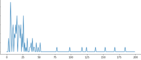
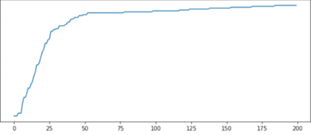
Figure 1: typical return incidence x days after a specific sale date.
Certain factors, however, make it hard to compare return rates with simple statistics, which is the reason why OTTO wants to use Data Science to get a better handle on return rates, predictions and action prioritization.
The Controlling Department has an elaborate tool to analyse return rates: 'RASY' tracks sales and returns for every OTTO (retail) product, together with the time it took between billing date and finalisation of the potential return.
The system analyses 'cohorts' of SKUs – assortments sold in the same month. The reason for this approach is, that the (realised) return rates of current cohorts always seems lower than previous ones, because OTTO allows returns within 30 days and in many cases much longer.
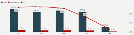
Figure 2: realised return rates of cohorts naturally drop as we get closer to the present
Figure 2 depicts this problem for a fictional article. Let’s assume today is May 10th. The months on the bottom represent the sales months of the article, with total sales in blue and absolute returns in red. While the sales numbers are already final for April and earlier, the returns aren’t yet, since many returns for products sold in April only arrive in May or even later. Thus the (realised) return rate (RQ) of April currently underestimates the final return rate. The effect for May is even stronger, in which neither sales nor returns are complete yet.
Thus, since a direct comparison of historic (realised) return rates (Jan, Feb, March) with current (realised) return rates makes no sense, Controlling makes super-complex comparisons with the past in the hope of finding significant deviations versus the forecast quickly. However, these comparisons are made on a shaky foundation, if we consider that the entire return chain doesn’t solely include the selection and examination of the product by the customer, but also contains 'noise' from delays in shipping and processing of returns due to holidays, Covid or strikes, among many other factors.
Our task was to model the final return rate for each sales month and SKU, which will be realised four months after each sales month is over. Four months is the absolute maximal timescale it takes until an article return is finalised, bearing the special conditions at OTTO which allow a 3-month return timeframe. Based on these estimates and their uncertainty intervals, OTTO Returns Managers can see quickly which SKUs are showing show abnormal behaviour – and then act fast.
Since it was a dear wish of OTTO Returns to keep RASY, which works on a sales-position level, our task was to enrich every single sales position with its return probability by the end of a four-month period after the sale date, together with an uncertainty measure. These statistics can then be dynamically aggregated on an SKU level and visualised in a time-series for the tool-user to spot abnormalities rapidly.
The nature of the problem (time-to-event data) calls for the 'survival analysis' toolbox. This is a field which started out in mortality modelling, but was quickly adopted in many other fields through simply replacing the event 'death' by any other event that seemed model-worthy – such as whether a sale ends in a return.
The idiosyncrasies of time-to-event data are that…
Products sold less than four months ago and not returned are called 'censored observations', since their final status still isn’t clear but they carry the information that the event hasn't occurred YET.
Together with the sale date and the return status (incl. return date), we also record features which help us in the modelling process. These contain, but are not limited to:
All in all, a dataset looking like Figure 3 below forms the basis of our modelling.
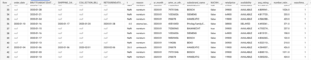
Figure 3: dataset
Multiple different survival models were trained and their performance on curated error measures were recorded using a three-month hold-out set.
*Non-parametric models only work on statistics based on empirical data; parametric models estimate weightings for each feature included in the model.
Another way to approach the problem of forecasting the final return rate would be to formulate it as a time-series problem. In particular, to decompose it into smaller time-series problems, which we can afterwards combine for the final forecasts.
More precisely, let's consider the final return rate that concerns sales on one specific day. Lining up all such rates in a daily fashion one after the other already provides us with a time-series to forecast what the next daily return rates could look like. It quickly becomes clear that restricting our approach to only the final return rates fails to take into account a key piece of information: the entire distribution of daily return rates over the possible timespan of the return period. Figure 1 offers an example of returns distribution.
Organizing these (density) distributions one after the other chronologically keeps much more of the original information intact and allows us to treat the problem as a functional time-series – one in which each time-step corresponds to a whole function (i.e. the distribution of daily return rates) rather than just one value (i.e. the total return rate).
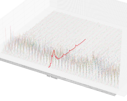
Figure 4: functional time-series. At each time-step we have the observed return density of sales on that particular day (one time-series for each sale date; one example highlighted in red).
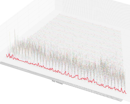
Figure 5: switch in time-series orientation, now modelling one time-series for each 'duration-time' (one example highlighted in red).
Figure 6 depicts the model’s forecast as a function of time* for ONE specific SKU, considering all sales in January 2022 to date. Even though the sales (let alone the returns) aren’t complete before 01 Feb. 2022, the model’s predictions (blue) are already fairly close to the final return rate (red). The uncertainty declines day by day as more and more data is fed in. Even before the sales month is over, the prediction never again deviates from the 'truth' (reality) more than 10% (a custom metric we call 'earliness') – and it appears that the truth was always within the Confidence boundary of the forecast. The realised return rate at the specific date is shown in black. We can easily see that this line does not approach the red one well until roughly 15 March.
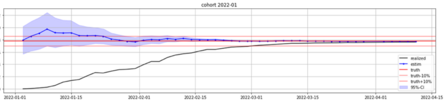
Figure 6: forecasts and errors
*This means that only data observed until this date is used to predict the final return rate (= 'truth' = red).
Aggregating these kinds of metrics was part of our model-selection scheme. To our surprise, the most basic model, Kaplan-Meyer, performed best on our metrics and was therefore the first model to be put into our pipeline in the first iteration. Our evaluation for this product class indicated that it takes on average only 8 days after the current month has ended for the model’s prediction not to deviate from the final return rate (of the month for an SKU) more than 1% pt.
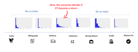
Figure 7: milestones in returns
Additionally, the collection date happens on average ~12 days before the finalisation date. Using this date, the status of our returns therefore become clear 12 days earlier, which yields higher confidence in our estimates faster.
The following graph in Figure 8 shows that the return hazard* using the collection date (blue) is much earlier (peaking at Day 3) than if we use the finalisation date (orange, peaking at Day 14).
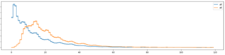
Figure 8: return-rate hazard, considering two different milestones
The first analyses indicate that using this approach will decrease our uncertainty intervals by approximately 30% and yield estimates of the same quality 12 days earlier than if we take the approach of iteration I.
Unfortunately, obtaining these necessary timestamps reliably for every return is complicated due to unexpected customer behaviour and the unaligned data structures of the various delivery companies OTTO works with.
*'hazard' means the probability of experiencing the 'event' exactly in the next timestep, given that the 'event' has not yet been experienced.
Together with every return, a return reason is also tracked in one of 6 main categories. These include problems with order/delivery, unsatisfactory quality, wrong size, and others.
A graph of the reason-specific survival-analysis hazard rates show these differ widely, and each is idiosyncratic for the respective category (Fashion vs Consumer Electronics vs Living).

Figure 9: return hazard for different risks
These graphs provide strong indications that it makes sense to model each of the reasons separately and not calculate one overall model. This could also be the reason why the feature-based approaches in iteration I yielded worse results than Kaplan-Meyer; the models had to estimate the influence of the features for all reasons at the same time, when for instance it is apparent on the one hand that the retail season or Covid restrictions will have a strong influence on the delivery-based return hazards (early hazard) but not on the quality, and on the other that serial production faults will strongly influence the quality-based return reason, yet leave the delivery (early hazard) rather untouched. For the Consumer Electronics article depicted here, size doesn’t play a role in return reasons at all.
Additionally, we have high hopes that combining time-series based models with survival-based models will achieve even better forecasting accuracy. We'll get back to you soon to shed more light on these topics!
Want to be part of our team?


We have received your feedback.


